Visualizing commodity trade in mercury with an interactive 3D globe

A data visualization app called Flourish has been getting a bit of buzz recently, so I decided to check it out. I noticed a slick existing template using 3D WebGL for illustrating global trade flows. I have a perfect dataset for that!

Our recently published UN Environment Global Mercury Supply, Trade and Demand Report contains data pulled from the UN Comtrade database on global mercury trade in 2008 and 2015. A few hours of data munging and it was ready to go into the template. Flourish also has a story feature which allows you to walk viewers through an interactive graphic. Sort of like a story map in GIS. Here is the result:

2018-06-27_140608

Click on the image to view the interactive story

A link to the graphic itself (without the story) is here.

One word of caution. No matter how slick a graphic looks and performs, it’s only worth as much as the underlying data. In this case, we know that UN Comtrade data for mercury has some serious flaws, including errors and missed reporting by importing and exporting countries, to say nothing of illegal trade (we discuss these issues in the report). Nevertheless we believe the data is still useful in providing an overview of global trade. But please keep the limitations in mind.

Advertisement

Mercury in Chlor-Alkali Plants Mapped with CartoDB

The other day I learned that wordpress.com now supports embeds of CartoDB maps. This is pretty cool, and it inspired me to finish up a little project that I’ve been tinkering with for a while, in order to try out the new feature.

By the way, CartoDB is a web mapping tool that I think is one of the best interfaces available for creating interactive maps. You can make great looking maps quickly and easily, but there is also enough functionality to do more advanced stuff, like mess around with the CSS code.

This map shows estimates of how much mercury is on site at chlor-alkali plants per country. It distinguishes between countries that ban the export of mercury and those that don’t. This is important because chlor-alkali plants often contain hundreds of tons of mercury. When the facilities close the mercury can enter the commodity market where it can be used in artisanal gold mining.

The size of the bubbles reflects how many tons of mercury are estimated to be in chlor-alkali facilities in each country. Scroll, zoom, hover, or click for more details. The data are from the UNEP Global Mercury Partnership chlor-alkali inventory.

Technical CartoDB note: In order to distinguish (by bubble color) countries with and without export bans, I made two layers from the data table. However, because each set had a different range of values, the scale for the bubble size was different for each color. To fix this I manually changed the bubble size distribution cutoffs in the CSS tab. Is there an easier solution that I am missing?

Oh yeah, this is how you do the embed.

The Rio Declaration and the Decline of Multilateral Environmental Agreements

It’s been quite some time since my last post. I have been busy with a young child, new job, and an international move. But I’m hoping to get back into posting and making visualizations on a regular basis.

The reason for this post is that I came across an interesting resource called the International Environmental Agreements Database Project, hosted at the University of Oregon. The database contains information on about 1100 multilateral environmental agreements (MEAs) dating back to 1857. The data include the title, type (an original agreement or a protocol or amendment to an existing agreement), dates of signature and entry into force, and the parties. For some agreements there is even data on performance as well as coding to allow for comparison of the actual legal components.

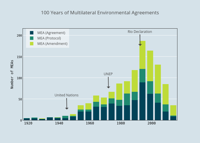
As an initial exploration, I simply looked at how many agreements were concluded over time. The plot below shows the results for the last 100 years. Click for the interactive and shareable plot.ly version.

100 Years of Multilateral Environmental Agreements

Click for interactive version

There is a pretty interesting pattern. From the early 20th century until the 1950s there are not that many MEAs. Then the pace picks up in mid-century, peaking in the early 1990s, and declining considerably after that.

What’s going on? Have all the easy agreements been reached and there is nothing more for countries to negotiate about? Maybe that’s part of it, but I think it has something to do with an event that coincided with the peak in MEAs – The 1992 Earth Summit and the resulting Rio Declaration on Environment and Development.

The Earth Summit was a huge event in the global environmental community, and occurred at a high point of optimism about multilateralism. There was a flurry of MEA activity around this time. But there was also a building movement to ensure that international environmental diplomacy was benefiting the poor, and in particular, developing countries.

The Rio Declaration enshrined the principle of common but differentiated responsibilities. This is the idea that while all nations have a responsibility to protect the global environment, rich nations should shoulder a greater share of the burden.

It is a noble sentiment, and one that in my view makes a lot of sense. But it had the effect of making it more difficult to reach agreements in international environmental negotiations. Developing countries started going into the negotiations expecting more support, in the form of funding, reduced obligations, or technology transfer, from the developed world. Common but differentiated responsibilities is at the root of a major sticking point in global climate talks. Should China, India, and other rapidly developing nations have the same stringent obligations as more mature economies?

I certainly don’t think this is the only cause of the decline in new MEAs in the last 20 years. And neither can I claim to be the first to think about the Rio Declaration’s impact on MEAs. There’s an entire literature on it. For example, Richard Benedick discussed this theme at length in reference to the Montreal Protocol and its aftermath in his book Ozone Diplomacy.

As a final disclaimer, for this analysis it would be best to filter the IEA database to exclude those MEAs that only have a few parties. That way you could really focus on the rate of global or large regional MEAs over time. Perhaps I’ll do that next.

But in any case, it’s an interesting dataset and an interesting pattern. And a good excuse to step back and think about the big picture in global environmental politics.

Using Tableau Public to Make an Interactive Visualization

Dashboard_1 For the last several weeks I’ve been experimenting with Tableau Public, a powerful, free software package for data analysis and visualization. I’m impressed by the software. It’s certainly the best free product I’ve worked with.

My big project on Tableau is an interactive graphic showing global mercury emissions by country and sector. I was able to get a nice dataset from the Arctic Monitoring and Assessment Program. These data were part of the 2013 UNEP Global Mercury Assessment. So they are very up-to-date, and with the adoption of the new Minamata Convention on Mercury, the topic is quite relevant. Good ingredients for an nice viz.

The graphic combines three elements: 1) a world map showing mercury emissions by country in a color gradient scale, 2) a tree map showing the mercury emissions of regions and their constituent countries as a part of total global emissions, and 3) a bar graph showing the makeup of emissions by industry sector for the world or selected countries. All the elements are linked so that selecting objects in one changes the other elements.

Check it out.